


SpaceX News
NASA requests proposals to reduce cost, timeline of Mars Sample Return mission – Spaceflight Now
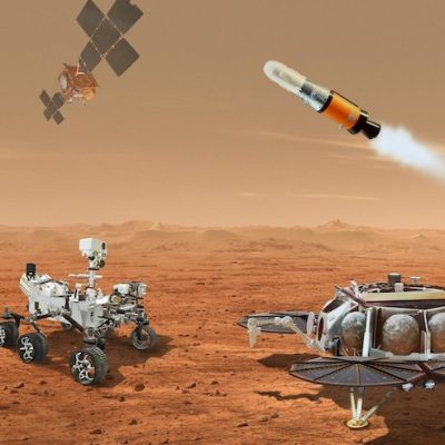
This illustration shows a concept for multiple robots that would team up to ferry to Earth samples of rocks and soil being collected from the Martian surface by NASA’s Mars Perseverance rover.Credit: NASA/ESA/JPL-Caltech...